Visualizing high-dimensional data with t-SNE
Guest author: thanks to Aviv Netanyahu for writing this post!
1 What is visualization and why do we need it?
Before working on a dataset we would like to understand it. After working on it, we want to communicate our conclusions with others easily. When dealing with high-dimensional data, it’s hard to get a ’feel’ for the data by just looking at numbers, and we will advance pretty slowly. For example, common visualization methods are histograms and scatter plots, which capture only one or two parameters at a time, meaning we would have to look at many histograms (one for each feature). However, by visualizing our data we may instantly be able to recognize structure. In order to do this we would like to find a representation of our data in
D or
D.
2 Our goal
Find an embedding of high-dimensional data to 2D or 3D (for simplicity, will assume
D from now on).
Formally, we want to learn ( is our data, is the embedding) such that the structure of the original data is preserved after the embedding.
Formally, we want to learn ( is our data, is the embedding) such that the structure of the original data is preserved after the embedding.
3 So why not PCA?
PCA projects high-dimensional data onto a lower dimension determined by the directions where the data varies most in. The result is a linear projection which focuses on preserving distance between dissimilar data points. This is problematic:
- Linear sometimes isn’t good enough.
- We claim structure is mostly determined by similar data points.
4 SNE (Hinton&Roweis)
This algorithm for high-dimensional data visualization focuses on preserving high-dimensional ’neighbors’ in low-dimension.
Assumption - ’neighbors’ in high dimension have small Euclidean distance. SNE converts the Euclidean distances to similarities using Gaussian distribution:
is the probability that
is the neighbor of
in high-dimension.
is the probability that
is the neighbor of
in low-dimension.
Note - choosing for is done by determining the perplexity, i.e. the effective number of neighbors for each data point. Then , is chosen such that has according number of neighbors in the multivariate Gaussian with mean and covariance matrix .
By mapping each to such that is close as possible to , we can preserve similarities. The algorithm finds such a mapping by gradient descent w.r.t. the following loss (cost) function: where and the initialization of low-dimensional data is random around the origin.
Notice the loss function, Kullback–Leibler (KL) divergence, is a natural way to measure similarity between two distributions.
Also notice that this loss puts more emphasis on preserving the local structure of the data. KL-div is asymmetric, so different kinds of errors have a different affect:
Also notice that this loss puts more emphasis on preserving the local structure of the data. KL-div is asymmetric, so different kinds of errors have a different affect:
- Type 1 error: is large (i.e. two points were originally close) and small (i.e. these points were mapped too far), we pay a large penalty.
- Type 2 error: is small (i.e. two points were originally far away) and large (i.e. these points were mapped too close), we pay a small penalty.
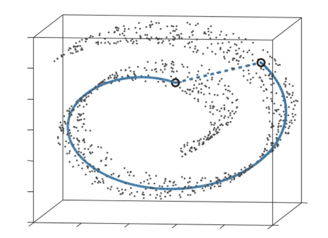
This is good, as structure is preserved better by focusing on keeping close points together. This is easy to see in the following example: think of “unrolling” this swiss roll (like unrolling a carpet). Close points will stay within the same distance, far points won’t. This is true for many manifolds (spaces that locally resemble Euclidean space near each point) besides the swiss roll.

4.1 The crowding problem
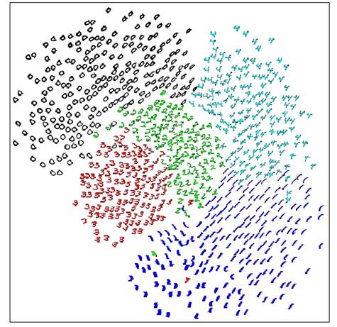
The main problem with SNE - mapped points tend to “crowd” together, like in this example: images of 5 MNIST digits mapped with SNE to 2D and then marked by labels

This happens because when reducing the dimensionality we need more “space” in which to represent our data-points. You can think of a sphere flattened to a circle where all distances are preserved (as much as possible) - the radius of the circle will have to be larger than the radius of the sphere!
On one hand this causes type
error (close points mapped too far), which forces far mapped points to come closer together. On the other, causes type
error (far points mapped close) which forces them to move away from each other. Type
error makes us pay a small price, however if many points cause error
, the price will be higher, forcing the points to indeed move. What we just described causes the mapped points to correct themselves to the center such that they end up very close to each other. Consider the MNIST example above. If we did not know the labels we couldn’t make much sense of the mapping.
5 T-SNE (van der Maaten&Hinton)
5.1 Solving the crowding problem
Instead of mapped points correcting themselves to minimize the loss, we can do this by increasing
in advance. Recall, the loss is:
, thus larger
minimizes it. We do this by defining:
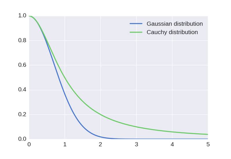
using Cauchy distribution instead of Gaussian distribution. This increases
since Cauchy distribution has a heavier tail than Gaussian distribution:

Note also that we changed the probability from conditional to joint probability (this was done for technical optimization reasons). For the same reason,
was converted to
. We can still use Gaussian distribution for the original data since we are trying to compensate for error in the mapped space.
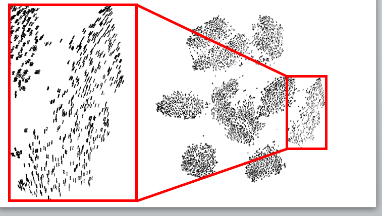
Now the performance on MNIST is much better:

It’s obvious that global structure is preserved and crowding is resolved. Notice also that when zooming in on the mapping of
digits, the local structure is preserved as well - digits with same orientation were mapped close to each other.
6 Barnes-Hut approximation (van der Maaten)
Computing the gradient for each mapped point each iteration is very costly, especially when the dataset is very large. At each iteration,
, we compute:
We can think of
as a spring between these two points (it might be too tight/loose depending on if the points were mapped to far/close accordingly). The fraction can be thought of as exertion/compression of the spring, in other words the correction we do in this iteration. We calculate this for
mapped points, and derive
by all data-points, so for each iteration we have
computations. This limits us to datasets with only few thousands of points! However, we can reduce the computation time to
by reducing the number of computations per iteration. The main idea - forces exerted by a group of points on a point that is relatively far away are all very similar. Therefore we can calculate
where
is the average of the group of far away points, instead of
for each
in the far away group.
7 Some applications
- Visualize word embeddings - http://nlp.yvespeirsman.be/blog/visualizing-word-embeddings-with-tsne/
- Multiple maps word embeddings - http://homepage.tudelft.nl/19j49/multiplemaps/Multiple_maps_t-SNE/Multiple_maps_t-SNE.html
- Visualization of genetic disease phenotype similarities by multiple maps t-SNE - https://www.ncbi.nlm.nih.gov/pmc/articles/PMC4243097/
8 When can t-SNE fail?
When the data is noisy or on a highly varying manifold, the local linearity assumption we make (by converting Euclidean distances to similarities) does not hold. What can we do? - smooth data with PCA (in case of noise) or use Autoencoders (in case of highly varying manifold).